What if you have a very small dataset of only a few thousand images and a hard classification problem at hand? Training a network from scratch might not work that well, but how about transfer learning.
Dog Breed Classification with Keras
Recently, I got my hands on a very interesting dataset that is part of the Udacity AI Nanodegree. In several of my previous posts I discussed the enormous potential of transfer learning. As a matter of fact, very few people train an entire convolutional network from scratch (with random initialization), because it is relatively rare to have a dataset of sufficient size. Instead, it is common to pre-train a convolutional network on a very large dataset (e.g. ImageNet, which contains 1.2 million images with 1000 categories), and then use the convolutional network either as an initialization or a fixed feature extractor for the task of interest.
In this post, I aim to compare two approaches to image classification. First, I will train a convolutional neural network from scratch and measure its performance. Then, I will apply transfer learning and will create a stack of models and compare their performance to the first approach. For that purpose, I will use Keras. While I got really comfortable at using Tensorflow, I must admit, using the high-level wrapper API that is Keras gets you much faster to the desired network architecture. Nevertheless, I still would recommend to every beginner to start with Tensorflow, as its low-level API really helps you understand how different types of neural networks work.
Dog Breed Dataset
The data consists of 8351 dog images. The images are sorted into 133 directories, each directory contains only images of a single dog breed. Hopefully, the dataset will stay here. If the url is not available, feel free to contact me. Ok, let’s load the dataset.
from sklearn.datasets import load_files
from keras.utils import np_utils
import numpy as np
from glob import glob

def load_dataset(path):
    data = load_files(path)
    dog_files = np.array(data['filenames'])
    dog_targets = np_utils.to_categorical(np.array(data['target']), 133)
    return dog_files, dog_targets

train_files, train_targets = load_dataset('dog/assets/images/train')
valid_files, valid_targets = load_dataset('dog/assets/images/valid')
test_files, test_targets = load_dataset('dog/assets/images/test')

dog_names = [item[20:-1] for item in sorted(glob("dog/assets/images/train/*/"))]

# Let's check the dataset
print('There are %d total dog categories.' % len(dog_names))
print('There are %s total dog images.\n' % len(np.hstack([train_files, valid_files, test_files])))
print('There are %d training dog images.' % len(train_files))
print('There are %d validation dog images.' % len(valid_files))
print('There are %d test dog images.'% len(test_files))
Using TensorFlow backend.

There are 133 total dog categories.
There are 8351 total dog images.

There are 6680 training dog images.
There are 835 validation dog images.
There are 836 test dog images.
The dataset is already split into train, validation and test parts. As the training set consists of 6680 images, there are only 50 dogs per breed on average. That is really a rather small dataset and an ambitious task to do. The cifar 10 dataset for example contains 60000 images and only 10 categories. The categories are airplane, automobile, bird, cat, etc. Thus, objects to be classified are very different and therefore easier to classify. In my post Image classification with pre-trained CNN InceptionV3 I managed to achieve an accuracy of around 80%. Hence, it is now my goal to achieve similar accuracy with the dog breed dataset, that has much more categories, while it is much much smaller.
Why is the dataset interesting?
The task of assigning breed to dogs from images is considered exceptionally challenging. To see why, consider that even a human would have great difficulty in distinguishing between a Brittany and a Welsh Springer Spaniel.
| Brittany | Welsh Springer Spaniel |
|---|---|
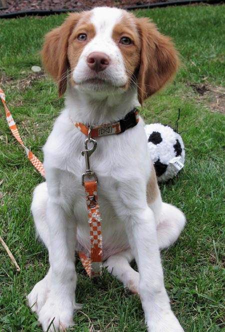 |
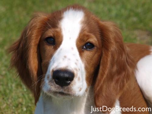 |
It was not difficult to find other dog breed pairs with only few inter-class variations (for instance, Curly-Coated Retrievers and American Water Spaniels).
| Curly-Coated Retriever | American Water Spaniel |
|---|---|
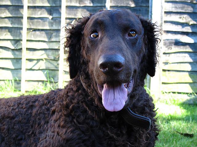 |
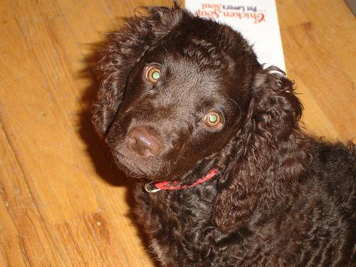 |
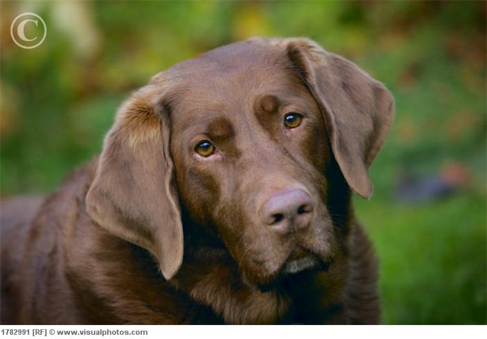
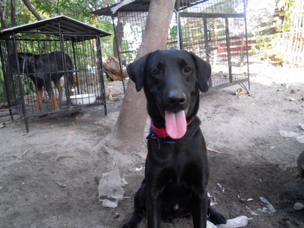
Likewise, labradors come in yellow, chocolate, and black. A vision-based algorithm will have to conquer this high intra-class variation to determine how to classify all of these different shades as the same breed.
| Yellow Labrador | Chocolate Labrador | Black Labrador |
|---|---|---|
 |
 |
 |
When predicting between 133 breeds, a random chance presents an exceptionally low bar: setting aside the fact that the classes are slightly imbalanced, a random guess will provide a correct answer roughly 1 in 133 times, which corresponds to an accuracy of less than 1%. Hence, even an accuracy of 2-3% would be considered reasonable.
Pre-process the Data
When using TensorFlow as backend, Keras CNNs require a 4D array (which we’ll also refer to as a 4D tensor) as input, with shape
where nb_samples corresponds to the total number of images (or samples), and rows, columns, and channels correspond to the number of rows, columns, and channels for each image, respectively.
The path_to_tensor function below takes a string-valued file path to a color image as input and returns a 4D tensor suitable for supplying to a Keras CNN. The function first loads the image and resizes it to a square image that is $224 \times 224$ pixels. Next, the image is converted to an array, which is then resized to a 4D tensor. In this case, since we are working with color images, each image has three channels. Likewise, since we are processing a single image (or sample), the returned tensor will always have shape
The paths_to_tensor function takes a numpy array of string-valued image paths as input and returns a 4D tensor with shape
Here, nb_samples is the number of samples, or number of images, in the supplied array of image paths. It is best to think of nb_samples as the number of 3D tensors (where each 3D tensor corresponds to a different image) in your dataset!
from keras.preprocessing import image
from tqdm import tqdm

def path_to_tensor(img_path):
    # loads RGB image as PIL.Image.Image type
    img = image.load_img(img_path, target_size=(224, 224))
    # convert PIL.Image.Image type to 3D tensor with shape (224, 224, 3)
    x = image.img_to_array(img)
    # convert 3D tensor to 4D tensor with shape (1, 224, 224, 3) and return 4D tensor
    return np.expand_dims(x, axis=0)

def paths_to_tensor(img_paths):
    list_of_tensors = [path_to_tensor(img_path) for img_path in tqdm(img_paths)]
    return np.vstack(list_of_tensors)
We rescale the images by dividing every pixel in every image by 255.
from PIL import ImageFile
ImageFile.LOAD_TRUNCATED_IMAGES = True

# pre-process the data for Keras
train_tensors = paths_to_tensor(train_files).astype('float32')/255
valid_tensors = paths_to_tensor(valid_files).astype('float32')/255
test_tensors = paths_to_tensor(test_files).astype('float32')/255
100%|██████████| 6680/6680 [01:00<00:00, 110.84it/s]
100%|██████████| 835/835 [00:06<00:00, 127.85it/s]
100%|██████████| 836/836 [00:06<00:00, 136.50it/s]
Create a CNN to Classify Dog Breeds (from Scratch)
After few hours of trial and error, I came up with the following CNN architecture:
from keras.layers import Conv2D, MaxPooling2D, GlobalAveragePooling2D
from keras.layers import Dropout, Activation, Dense
from keras.models import Sequential
from keras.layers.normalization import BatchNormalization

model = Sequential()

model.add(Conv2D(16, (3, 3), padding='same', use_bias=False, input_shape=(224, 224, 3)))
model.add(BatchNormalization(axis=3, scale=False))
model.add(Activation("relu"))
model.add(MaxPooling2D(pool_size=(4, 4), strides=(4, 4), padding='same'))
model.add(Dropout(0.2))

model.add(Conv2D(32, (3, 3), padding='same', use_bias=False))
model.add(BatchNormalization(axis=3, scale=False))
model.add(Activation("relu"))
model.add(MaxPooling2D(pool_size=(4, 4), strides=(4, 4), padding='same'))
model.add(Dropout(0.2))

model.add(Conv2D(64, (3, 3), padding='same', use_bias=False))
model.add(BatchNormalization(axis=3, scale=False))
model.add(Activation("relu"))
model.add(MaxPooling2D(pool_size=(4, 4), strides=(4, 4), padding='same'))
model.add(Dropout(0.2))

model.add(Conv2D(128, (3, 3), padding='same', use_bias=False))
model.add(BatchNormalization(axis=3, scale=False))
model.add(Activation("relu"))
model.add(Flatten())
model.add(Dropout(0.2))

model.add(Dense(512, activation='relu'))
model.add(Dense(133, activation='softmax'))
model.summary()
_________________________________________________________________
Layer (type)                 Output Shape              Param #
=================================================================
conv2d_46 (Conv2D)           (None, 224, 224, 16)      432
_________________________________________________________________
batch_normalization_105 (Bat (None, 224, 224, 16)      48
_________________________________________________________________
activation_1479 (Activation) (None, 224, 224, 16)      0
_________________________________________________________________
max_pooling2d_66 (MaxPooling (None, 56, 56, 16)        0
_________________________________________________________________
dropout_84 (Dropout)         (None, 56, 56, 16)        0
_________________________________________________________________
conv2d_47 (Conv2D)           (None, 56, 56, 32)        4608
_________________________________________________________________
batch_normalization_106 (Bat (None, 56, 56, 32)        96
_________________________________________________________________
activation_1480 (Activation) (None, 56, 56, 32)        0
_________________________________________________________________
max_pooling2d_67 (MaxPooling (None, 14, 14, 32)        0
_________________________________________________________________
dropout_85 (Dropout)         (None, 14, 14, 32)        0
_________________________________________________________________
conv2d_48 (Conv2D)           (None, 14, 14, 64)        18432
_________________________________________________________________
batch_normalization_107 (Bat (None, 14, 14, 64)        192
_________________________________________________________________
activation_1481 (Activation) (None, 14, 14, 64)        0
_________________________________________________________________
max_pooling2d_68 (MaxPooling (None, 4, 4, 64)          0
_________________________________________________________________
dropout_86 (Dropout)         (None, 4, 4, 64)          0
_________________________________________________________________
conv2d_49 (Conv2D)           (None, 4, 4, 128)         73728
_________________________________________________________________
batch_normalization_108 (Bat (None, 4, 4, 128)         384
_________________________________________________________________
activation_1482 (Activation) (None, 4, 4, 128)         0
_________________________________________________________________
flatten_2 (Flatten)          (None, 2048)              0
_________________________________________________________________
dropout_87 (Dropout)         (None, 2048)              0
_________________________________________________________________
dense_100 (Dense)            (None, 512)               1049088
_________________________________________________________________
dense_101 (Dense)            (None, 133)               68229
=================================================================
Total params: 1,215,237
Trainable params: 1,214,757
Non-trainable params: 480
_________________________________________________________________
As already elaborated, designing a CNN architecture that achieves even 2% accuracy is not an easy task. The first thing you notice is that increasing the filters depth leads to better results, yet slower training.Batch Normalization seems not only to lead to faster training, but also to better results. I used the source code of InceptionV3 as an example when configuring the batch normalization layers. As batch normalization allowed for the model to learn much faster and I added a fourth convolutional layer and further increased the filter depth. Then, I altered the max pooling layer to shrink the layers by a factor of x4 instead of x2. This drastically decreased the number of trainable params and increased the speed by which the model is learning. At the end I added Dropout, to decrease overfitting, as the network started to overfit after the 4th epoch.
from keras.callbacks import ModelCheckpoint

EPOCHS = 10
model.compile(optimizer='rmsprop', loss='categorical_crossentropy', metrics=['accuracy'])
checkpointer = ModelCheckpoint(filepath='saved_models/weights.best.from_scratch.hdf5',
                               verbose=1, save_best_only=True)
model.fit(train_tensors, train_targets,
          validation_data=(valid_tensors, valid_targets),
          epochs=EPOCHS, batch_size=32, callbacks=[checkpointer], verbose=1)
Train on 6680 samples, validate on 835 samples
Epoch 1/10
6656/6680 [============================>.] - ETA: 1s - loss: 4.8959 - acc: 0.0207Epoch 00000: val_loss improved from inf to 5.09728, saving model to saved_models/weights.best.from_scratch.hdf5
6680/6680 [==============================] - 434s - loss: 4.8946 - acc: 0.0207 - val_loss: 5.0973 - val_acc: 0.0156
Epoch 2/10
6656/6680 [============================>.] - ETA: 0s - loss: 4.4014 - acc: 0.0524Epoch 00001: val_loss improved from 5.09728 to 4.45084, saving model to saved_models/weights.best.from_scratch.hdf5
6680/6680 [==============================] - 292s - loss: 4.4012 - acc: 0.0524 - val_loss: 4.4508 - val_acc: 0.0479
Epoch 3/10
6656/6680 [============================>.] - ETA: 0s - loss: 4.1037 - acc: 0.0726Epoch 00002: val_loss did not improve
6680/6680 [==============================] - 274s - loss: 4.1032 - acc: 0.0731 - val_loss: 4.4804 - val_acc: 0.0443
Epoch 4/10
6656/6680 [============================>.] - ETA: 0s - loss: 3.9247 - acc: 0.0959Epoch 00003: val_loss improved from 4.45084 to 4.43195, saving model to saved_models/weights.best.from_scratch.hdf5
6680/6680 [==============================] - 273s - loss: 3.9240 - acc: 0.0960 - val_loss: 4.4319 - val_acc: 0.0491
Epoch 5/10
6656/6680 [============================>.] - ETA: 0s - loss: 3.7687 - acc: 0.1175Epoch 00004: val_loss did not improve
6680/6680 [==============================] - 276s - loss: 3.7678 - acc: 0.1175 - val_loss: 4.9665 - val_acc: 0.0347
Epoch 6/10
6656/6680 [============================>.] - ETA: 0s - loss: 3.6533 - acc: 0.1315Epoch 00005: val_loss did not improve
6680/6680 [==============================] - 293s - loss: 3.6520 - acc: 0.1317 - val_loss: 4.6552 - val_acc: 0.0671
Epoch 7/10
6656/6680 [============================>.] - ETA: 1s - loss: 3.5410 - acc: 0.1513Epoch 00006: val_loss improved from 4.43195 to 4.18182, saving model to saved_models/weights.best.from_scratch.hdf5
6680/6680 [==============================] - 313s - loss: 3.5407 - acc: 0.1510 - val_loss: 4.1818 - val_acc: 0.0743
Epoch 8/10
6656/6680 [============================>.] - ETA: 1s - loss: 3.4297 - acc: 0.1773Epoch 00007: val_loss improved from 4.18182 to 4.05759, saving model to saved_models/weights.best.from_scratch.hdf5
6680/6680 [==============================] - 310s - loss: 3.4286 - acc: 0.1772 - val_loss: 4.0576 - val_acc: 0.1066
Epoch 9/10
6656/6680 [============================>.] - ETA: 1s - loss: 3.3242 - acc: 0.1881Epoch 00008: val_loss did not improve
6680/6680 [==============================] - 297s - loss: 3.3236 - acc: 0.1883 - val_loss: 4.4697 - val_acc: 0.0683
Epoch 10/10
6656/6680 [============================>.] - ETA: 1s - loss: 3.1783 - acc: 0.2160Epoch 00009: val_loss did not improve
6680/6680 [==============================] - 300s - loss: 3.1793 - acc: 0.2156 - val_loss: 4.2501 - val_acc: 0.1006
Running the model for 10 epochs took less than an hour, when running on 8-Core CPU. Meanwhile, I am using Floyd Hub to rent a GPU when considerably more power is required. In mostly works fine, once you manage to upload your dataset (their upload pipeline is currently buggy). Let’s load the weights of the model that had the best validation loss and measure the accuracy.
model.load_weights('saved_models/weights.best.from_scratch.hdf5')
# get index of predicted dog breed for each image in test set
dog_breed_predictions = [np.argmax(model.predict(np.expand_dims(tensor, axis=0))) for tensor in test_tensors]
# report test accuracy
test_accuracy = 100*np.sum(np.array(dog_breed_predictions)==np.argmax(test_targets, axis=1))/len(dog_breed_predictions)
print('Test accuracy: %.4f%%' % test_accuracy)
Test accuracy: 11.1244%
That is not a bad performance. Probably as good as someone that is not an expert, but really likes dogs would manage to achieve.
Using pre-trained VGG-19 and Resnet-50
Next, we will use transfer learning to create a CNN that can identify dog breed from images. The model uses the pre-trained VGG-19 and Resnet-50 models as a fixed feature extractor, where the last convolutional output of both networks is fed as input to another, second level model. As a matter of fact, one can choose between several pre-trained models that are shipped with Keras. I have already tested VGG-16, VGG-19, InceptionV3, Resnet-50 and Xception on this dataset and found VGG-19 and Resnet-50 to have the best performance considering the limited memory resources and training time that I had at my disposal. At the end, I combined both models to achieve a small boost relative to what I achieved by using them separately. Here are few lines, that extract the features from the images:
We only add a global average pooling layer and a fully connected layer, where the latter contains one node for each dog category and is equipped with a softmax. Let’s extract the last convolutional output for both networks.
from keras.applications.vgg19 import VGG19
from keras.applications.vgg19 import preprocess_input as preprocess_input_vgg19
from keras.applications.resnet50 import ResNet50
from keras.applications.resnet50 import preprocess_input as preprocess_input_resnet50

def extract_VGG19(file_paths):
    tensors = paths_to_tensor(file_paths).astype('float32')
    preprocessed_input = preprocess_input_vgg19(tensors)
    return VGG19(weights='imagenet', include_top=False).predict(preprocessed_input, batch_size=32)

def extract_Resnet50(file_paths):
    tensors = paths_to_tensor(file_paths).astype('float32')
    preprocessed_input = preprocess_input_resnet50(tensors)
    return ResNet50(weights='imagenet', include_top=False).predict(preprocessed_input, batch_size=32)
Extracting the features may take a few minutes…
train_vgg19 = extract_VGG19(train_files)
valid_vgg19 = extract_VGG19(valid_files)
test_vgg19 = extract_VGG19(test_files)
print("VGG19 shape", train_vgg19.shape[1:])

train_resnet50 = extract_Resnet50(train_files)
valid_resnet50 = extract_Resnet50(valid_files)
test_resnet50 = extract_Resnet50(test_files)
print("Resnet50 shape", train_resnet50.shape[1:])
VGG19 shape (7, 7, 512)
Resnet50 shape (1, 1, 2048)
For the second level model, Batch Normalization yet again proved to be very important. Without batch normalization the model will not reach 80% accuracy for 10 epochs. Dropout is also important as it allows for the model to train more epochs before starting to overfit. However a Dropout of 50% leads to a model that trains all 20 epochs without overfitting, yet does not reach 82% accuracy. I’ve found Dropout of 30% to be just right for the model below. Another important hyper parameter was the batch size. A bigger batch size leads to a model that learns faster, the accuracy increases very rapidly, but the maximum accuracy is a bit lower. A smaller batch size leads to a model that learns slower between epochs but reaches higher accuracy.
from keras.layers.pooling import GlobalAveragePooling2D
from keras.layers.merge import Concatenate
from keras.layers import Input, Dense
from keras.layers.core import Dropout, Activation
from keras.callbacks import ModelCheckpoint
from keras.layers.normalization import BatchNormalization
from keras.models import Model

def input_branch(input_shape=None):

    size = int(input_shape[2] / 4)

    branch_input = Input(shape=input_shape)
    branch = GlobalAveragePooling2D()(branch_input)
    branch = Dense(size, use_bias=False, kernel_initializer='uniform')(branch)
    branch = BatchNormalization()(branch)
    branch = Activation("relu")(branch)
    return branch, branch_input

vgg19_branch, vgg19_input = input_branch(input_shape=(7, 7, 512))
resnet50_branch, resnet50_input = input_branch(input_shape=(1, 1, 2048))
concatenate_branches = Concatenate()([vgg19_branch, resnet50_branch])
net = Dropout(0.3)(concatenate_branches)
net = Dense(640, use_bias=False, kernel_initializer='uniform')(net)
net = BatchNormalization()(net)
net = Activation("relu")(net)
net = Dropout(0.3)(net)
net = Dense(133, kernel_initializer='uniform', activation="softmax")(net)

model = Model(inputs=[vgg19_input, resnet50_input], outputs=[net])
model.summary()
____________________________________________________________________________________________________
Layer (type)                     Output Shape          Param #     Connected to
====================================================================================================
input_3 (InputLayer)             (None, 7, 7, 512)     0
____________________________________________________________________________________________________
input_4 (InputLayer)             (None, 1, 1, 2048)    0
____________________________________________________________________________________________________
global_average_pooling2d_3 (Glob (None, 512)           0           input_3[0][0]
____________________________________________________________________________________________________
global_average_pooling2d_4 (Glob (None, 2048)          0           input_4[0][0]
____________________________________________________________________________________________________
dense_5 (Dense)                  (None, 128)           65536       global_average_pooling2d_3[0][0]
____________________________________________________________________________________________________
dense_6 (Dense)                  (None, 512)           1048576     global_average_pooling2d_4[0][0]
____________________________________________________________________________________________________
batch_normalization_4 (BatchNorm (None, 128)           512         dense_5[0][0]
____________________________________________________________________________________________________
batch_normalization_5 (BatchNorm (None, 512)           2048        dense_6[0][0]
____________________________________________________________________________________________________
activation_4 (Activation)        (None, 128)           0           batch_normalization_4[0][0]
____________________________________________________________________________________________________
activation_5 (Activation)        (None, 512)           0           batch_normalization_5[0][0]
____________________________________________________________________________________________________
concatenate_2 (Concatenate)      (None, 640)           0           activation_4[0][0]
                                                                   activation_5[0][0]
____________________________________________________________________________________________________
dropout_3 (Dropout)              (None, 640)           0           concatenate_2[0][0]
____________________________________________________________________________________________________
dense_7 (Dense)                  (None, 640)           409600      dropout_3[0][0]
____________________________________________________________________________________________________
batch_normalization_6 (BatchNorm (None, 640)           2560        dense_7[0][0]
____________________________________________________________________________________________________
activation_6 (Activation)        (None, 640)           0           batch_normalization_6[0][0]
____________________________________________________________________________________________________
dropout_4 (Dropout)              (None, 640)           0           activation_6[0][0]
____________________________________________________________________________________________________
dense_8 (Dense)                  (None, 133)           85253       dropout_4[0][0]
====================================================================================================
Total params: 1,614,085
Trainable params: 1,611,525
Non-trainable params: 2,560
____________________________________________________________________________________________________
model.compile(loss='categorical_crossentropy', optimizer="rmsprop", metrics=['accuracy'])
checkpointer = ModelCheckpoint(filepath='saved_models/bestmodel.hdf5',
                               verbose=1, save_best_only=True)
model.fit([train_vgg19, train_resnet50], train_targets,
          validation_data=([valid_vgg19, valid_resnet50], valid_targets),
          epochs=10, batch_size=4, callbacks=[checkpointer], verbose=1)
Train on 6680 samples, validate on 835 samples
Epoch 1/10
6676/6680 [============================>.] - ETA: 0s - loss: 2.5900 - acc: 0.3751Epoch 00000: val_loss improved from inf to 1.06250, saving model to saved_models/bestmodel.hdf5
6680/6680 [==============================] - 69s - loss: 2.5887 - acc: 0.3754 - val_loss: 1.0625 - val_acc: 0.6838
Epoch 2/10
6672/6680 [============================>.] - ETA: 0s - loss: 1.5383 - acc: 0.5679Epoch 00001: val_loss improved from 1.06250 to 0.87527, saving model to saved_models/bestmodel.hdf5
6680/6680 [==============================] - 50s - loss: 1.5376 - acc: 0.5680 - val_loss: 0.8753 - val_acc: 0.7401
Epoch 3/10
6676/6680 [============================>.] - ETA: 0s - loss: 1.3559 - acc: 0.6257Epoch 00002: val_loss improved from 0.87527 to 0.79809, saving model to saved_models/bestmodel.hdf5
6680/6680 [==============================] - 50s - loss: 1.3568 - acc: 0.6256 - val_loss: 0.7981 - val_acc: 0.7784
Epoch 4/10
6676/6680 [============================>.] - ETA: 0s - loss: 1.2502 - acc: 0.6552Epoch 00003: val_loss improved from 0.79809 to 0.74536, saving model to saved_models/bestmodel.hdf5
6680/6680 [==============================] - 49s - loss: 1.2503 - acc: 0.6551 - val_loss: 0.7454 - val_acc: 0.8012
Epoch 5/10
6676/6680 [============================>.] - ETA: 0s - loss: 1.1436 - acc: 0.6824Epoch 00004: val_loss did not improve
6680/6680 [==============================] - 49s - loss: 1.1438 - acc: 0.6823 - val_loss: 0.7806 - val_acc: 0.8084
Epoch 6/10
6672/6680 [============================>.] - ETA: 0s - loss: 1.0829 - acc: 0.7052Epoch 00005: val_loss improved from 0.74536 to 0.72584, saving model to saved_models/bestmodel.hdf5
6680/6680 [==============================] - 49s - loss: 1.0820 - acc: 0.7054 - val_loss: 0.7258 - val_acc: 0.8024
Epoch 7/10
6672/6680 [============================>.] - ETA: 0s - loss: 1.0586 - acc: 0.7136Epoch 00006: val_loss did not improve
6680/6680 [==============================] - 48s - loss: 1.0578 - acc: 0.7136 - val_loss: 0.7493 - val_acc: 0.8072
Epoch 8/10
6676/6680 [============================>.] - ETA: 0s - loss: 1.0034 - acc: 0.7218Epoch 00007: val_loss did not improve
6680/6680 [==============================] - 52s - loss: 1.0041 - acc: 0.7217 - val_loss: 0.7958 - val_acc: 0.8120
Epoch 9/10
6676/6680 [============================>.] - ETA: 0s - loss: 0.9489 - acc: 0.7326Epoch 00008: val_loss improved from 0.72584 to 0.72160, saving model to saved_models/bestmodel.hdf5
6680/6680 [==============================] - 47s - loss: 0.9484 - acc: 0.7328 - val_loss: 0.7216 - val_acc: 0.8228
Epoch 10/10
6676/6680 [============================>.] - ETA: 0s - loss: 0.9080 - acc: 0.7431Epoch 00009: val_loss did not improve
6680/6680 [==============================] - 47s - loss: 0.9076 - acc: 0.7433 - val_loss: 0.7365 - val_acc: 0.8228
Training the model takes only a few minutes… Let’s load the weights of the model that had the best validation loss and measure the accuracy.
model.load_weights('saved_models/bestmodel.hdf5')

from sklearn.metrics import accuracy_score

predictions = model.predict([test_vgg19, test_resnet50])
breed_predictions = [np.argmax(prediction) for prediction in predictions]
breed_true_labels = [np.argmax(true_label) for true_label in test_targets]
print('Test accuracy: %.4f%%' % (accuracy_score(breed_true_labels, breed_predictions) * 100))
Test accuracy: 82.2967%
The accuracy, when tested on the test set, is 82.3%. I find it really impressive compared to the 11% accuracy achieved by the model that was trained from scratch. The reason the accuracy is so much higher is that both VGG-19 and Resnet-50 were trained on ImageNet, which is not only huge (1.2 million images), but also contains a considerable amount of dog images. As a result, the accuracy achieved by using models pre-trained on ImageNet is much higher than the accuracy that could possibly be achieved by training a model from scratch. Well, Andrew Ng, the founder of Coursera and one of the biggest names in the ML realm said during his widely popular NIPS 2016 tutorial that transfer learning will be the next driver of ML commercial success. I can imagine, that in the future, models pre-trained on massive datasets would be made available by Google, Apple, Amazon, and others in exchange for some kind of subscription fee or some other form of payment. As a result, data scientists would be able to achieve remarkable results even when only provided with a limited set of data to use for training.
As always feel free to contact me or check out and execute the whole jupyter notebook: Dog Breed Github Repo