Google, Microsoft, and other vendors have been training very complex, state of the art Convolutional Neural Networks on massive datasets. In this post, I will explore “Transfer learning” - a very powerful bundle of techniques for reusing these already fully-trained neural networks for classification of images that can be more or less different from the images that have been used in the process of training those networks.
Image Classification with fine-tuned GoogleLeNet
In my previous post Convolutional neural network for image classification from scratch I built a small convolutional neural network (CNN) to classify images from the CIFAR-10 dataset. My goal was to demonstrate how easy one can construct a neural network with decent accuracy (around 67%). However, for many real word problems building CNNs from scratch might not be practical. For instance, in a recent kaggle challenge called Dog vs Cat the competitors were asked to correctly classify images of dogs and cats. In an insightful interview the winner of that challenge explained that he didn’t rely solely on a CNN that he built from scratch. Instead, he got his hands on multiple models already trained with large datasets and applied some “fine-tuning” in order to make these fit for the specific goal of classifying cats and dogs. So how does this work? The idea is simple. There are hundreds of models already trained on a specific dataset. The largest repository I know is the Model Zoo Github Repo. There are also the models from the Tensorflow Slim Project. So the goal is to select a model that is already trained on a dataset that is similar to the one you are interested in. After selecting the model one has to apply some “fine-tuning” on it. Interested? Well, continue reading, as this is exactly what I am going to do in this post.
Cifar-10 Image Dataset
If you are already familiar with my previous post Convolutional neural network for image classification from scratch, you might want to skip the next sections and go directly to Converting datasets to .tfrecord.
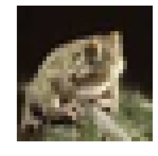
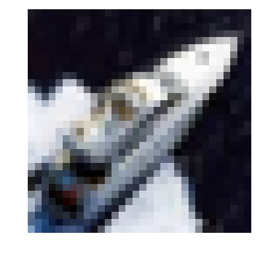
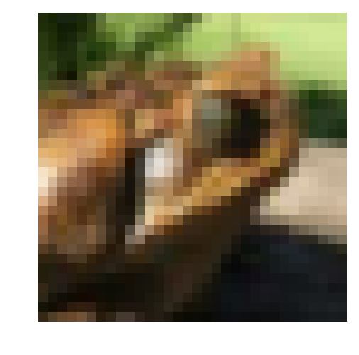
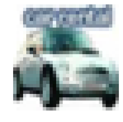
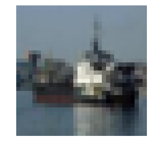
The CIFAR-10 dataset consists of 60000 32x32 color images in 10 categories - airplanes, dogs, cats, and other objects. The dataset is divided into five training batches and one test batch, each with 10000 images. The test batch contains exactly 1000 randomly-selected images from each class. The training batches contain the remaining images in random order, but some training batches may contain more images from one class than another. Between them, the training batches contain exactly 5000 images from each class. Here are the classes in the dataset, as well as 10 random images from each:
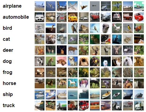
The classes are completely mutually exclusive. There is no overlap between automobiles and trucks. “Automobile” includes sedans, SUVs, things of that sort. “Truck” includes only big trucks. Neither includes pickup trucks.
Download the dataset
First, few lines of code will download the CIFAR-10 dataset for python.
# DOWNLOAD DATASET
from urllib.request import urlretrieve
import os
from tqdm import tqdm
import tarfile

class DLProgress(tqdm):
    last_block = 0

    def hook(self, block_num=1, block_size=1, total_size=None):
        self.total = total_size
        self.update((block_num - self.last_block) * block_size)
        self.last_block = block_num

if not os.path.isfile('cifar-10-python.tar.gz'):
    with DLProgress(unit='B', unit_scale=True, miniters=1, desc='CIFAR-10 Dataset') as pbar:
        urlretrieve(
            'https://www.cs.toronto.edu/~kriz/cifar-10-python.tar.gz',
            'cifar-10-python.tar.gz',
            pbar.hook)

if not os.path.isdir('cifar-10-batches-py'):
    with tarfile.open('cifar-10-python.tar.gz') as tar:
        tar.extractall()
        tar.close()
Data Overview
The dataset is broken into batches - this is especially useful if one is to train the network on a laptop as it will probably prevent it from running out of memory. I only had 12 GB on mine and a single batch used around 3.2 GB - it wouldn’t be possible to load everything at once. Nevertheless, the CIFAR-10 dataset consists of 5 batches, named data_batch_1, data_batch_2, etc.. Each batch contains the labels and images that are one of the following:
- airplane
- automobile
- bird
- cat
- deer
- dog
- frog
- horse
- ship
- truck
Understanding a dataset is part of making predictions on the data. Following functions can be used to view different images by changing the batch_id and sample_id. The batch_id is the id for a batch (1-5). The sample_id is the id for an image and label pair in the batch.
import pickle
import matplotlib.pyplot as plt

# The names of the classes in the dataset.
CLASS_NAMES = [
    'airplane',
    'automobile',
    'bird',
    'cat',
    'deer',
    'dog',
    'frog',
    'horse',
    'ship',
    'truck',
]

def load_cfar10_batch(batch_id):

    with open(os.path.join('cifar-10-batches-py','data_batch_'
              + str(batch_id)), mode='rb') as file:
        batch = pickle.load(file, encoding='latin1')

    features = batch['data'].reshape((len(batch['data']), 3, 32, 32)).transpose(0, 2, 3, 1)
    labels = batch['labels']

    return features, labels


def display_stats(features, labels, sample_id):

    if not (0 <= sample_id < len(features)):
        print('{} samples in batch {}.  {} is out of range.'
              .format(len(features), batch_id, sample_id))
        return None

    print('\nStats of batch {}:'.format(batch_id))
    print('Samples: {}'.format(len(features)))
    print('Label Counts: {}'.format(dict(zip(*np.unique(labels, return_counts=True)))))
    print('First 20 Labels: {}'.format(labels[:20]))

    sample_image = features[sample_id]
    sample_label = labels[sample_id]

    print('\nExample of Image {}:'.format(sample_id))
    print('Image - Min Value: {} Max Value: {}'.format(sample_image.min(), sample_image.max()))
    print('Image - Shape: {}'.format(sample_image.shape))
    print('Label - Label Id: {} Name: {}'.format(sample_label, CLASS_NAMES[sample_label]))
    plt.axis('off')
    plt.imshow(sample_image)
    plt.show()
Let’s check the first couple of images of each batch. The lines below can be easily modified to show an arbitrary image from any batch.
%matplotlib inline
%config InlineBackend.figure_format = 'retina'

import numpy as np

for batch_id in range(1,6):
    features, labels = load_cfar10_batch(batch_id)
    for image_id in range(0,2):
        display_stats(features, labels, image_id)

del features, labels # free memory
Stats of batch 1:
Samples: 10000
Label Counts: {0: 1005, 1: 974, 2: 1032, 3: 1016, 4: 999, 5: 937, 6: 1030, 7: 1001, 8: 1025, 9: 981}
First 20 Labels: [6, 9, 9, 4, 1, 1, 2, 7, 8, 3, 4, 7, 7, 2, 9, 9, 9, 3, 2, 6]
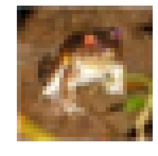
Example of Image 0:
Image - Min Value: 0 Max Value: 255
Image - Shape: (32, 32, 3)
Label - Label Id: 6 Name: frog
Stats of batch 1:
Samples: 10000
Label Counts: {0: 1005, 1: 974, 2: 1032, 3: 1016, 4: 999, 5: 937, 6: 1030, 7: 1001, 8: 1025, 9: 981}
First 20 Labels: [6, 9, 9, 4, 1, 1, 2, 7, 8, 3, 4, 7, 7, 2, 9, 9, 9, 3, 2, 6]
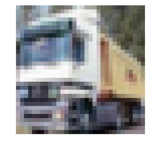
Example of Image 1:
Image - Min Value: 5 Max Value: 254
Image - Shape: (32, 32, 3)
Label - Label Id: 9 Name: truck
Stats of batch 2:
Samples: 10000
Label Counts: {0: 984, 1: 1007, 2: 1010, 3: 995, 4: 1010, 5: 988, 6: 1008, 7: 1026, 8: 987, 9: 985}
First 20 Labels: [1, 6, 6, 8, 8, 3, 4, 6, 0, 6, 0, 3, 6, 6, 5, 4, 8, 3, 2, 6]
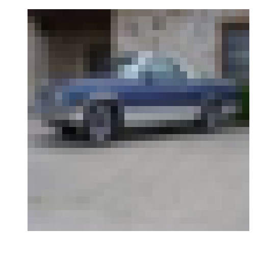
Example of Image 0:
Image - Min Value: 5 Max Value: 225
Image - Shape: (32, 32, 3)
Label - Label Id: 1 Name: automobile
Stats of batch 2:
Samples: 10000
Label Counts: {0: 984, 1: 1007, 2: 1010, 3: 995, 4: 1010, 5: 988, 6: 1008, 7: 1026, 8: 987, 9: 985}
First 20 Labels: [1, 6, 6, 8, 8, 3, 4, 6, 0, 6, 0, 3, 6, 6, 5, 4, 8, 3, 2, 6]

Example of Image 1:
Image - Min Value: 2 Max Value: 247
Image - Shape: (32, 32, 3)
Label - Label Id: 6 Name: frog
Stats of batch 3:
Samples: 10000
Label Counts: {0: 994, 1: 1042, 2: 965, 3: 997, 4: 990, 5: 1029, 6: 978, 7: 1015, 8: 961, 9: 1029}
First 20 Labels: [8, 5, 0, 6, 9, 2, 8, 3, 6, 2, 7, 4, 6, 9, 0, 0, 7, 3, 7, 2]

Example of Image 0:
Image - Min Value: 0 Max Value: 254
Image - Shape: (32, 32, 3)
Label - Label Id: 8 Name: ship
Stats of batch 3:
Samples: 10000
Label Counts: {0: 994, 1: 1042, 2: 965, 3: 997, 4: 990, 5: 1029, 6: 978, 7: 1015, 8: 961, 9: 1029}
First 20 Labels: [8, 5, 0, 6, 9, 2, 8, 3, 6, 2, 7, 4, 6, 9, 0, 0, 7, 3, 7, 2]

Example of Image 1:
Image - Min Value: 15 Max Value: 249
Image - Shape: (32, 32, 3)
Label - Label Id: 5 Name: dog
Stats of batch 4:
Samples: 10000
Label Counts: {0: 1003, 1: 963, 2: 1041, 3: 976, 4: 1004, 5: 1021, 6: 1004, 7: 981, 8: 1024, 9: 983}
First 20 Labels: [0, 6, 0, 2, 7, 2, 1, 2, 4, 1, 5, 6, 6, 3, 1, 3, 5, 5, 8, 1]

Example of Image 0:
Image - Min Value: 34 Max Value: 203
Image - Shape: (32, 32, 3)
Label - Label Id: 0 Name: airplane

Stats of batch 4:
Samples: 10000
Label Counts: {0: 1003, 1: 963, 2: 1041, 3: 976, 4: 1004, 5: 1021, 6: 1004, 7: 981, 8: 1024, 9: 983}
First 20 Labels: [0, 6, 0, 2, 7, 2, 1, 2, 4, 1, 5, 6, 6, 3, 1, 3, 5, 5, 8, 1]

Example of Image 1:
Image - Min Value: 0 Max Value: 246
Image - Shape: (32, 32, 3)
Label - Label Id: 6 Name: frog
Stats of batch 5:
Samples: 10000
Label Counts: {0: 1014, 1: 1014, 2: 952, 3: 1016, 4: 997, 5: 1025, 6: 980, 7: 977, 8: 1003, 9: 1022}
First 20 Labels: [1, 8, 5, 1, 5, 7, 4, 3, 8, 2, 7, 2, 0, 1, 5, 9, 6, 2, 0, 8]

Example of Image 0:
Image - Min Value: 2 Max Value: 255
Image - Shape: (32, 32, 3)
Label - Label Id: 1 Name: automobile
Stats of batch 5:
Samples: 10000
Label Counts: {0: 1014, 1: 1014, 2: 952, 3: 1016, 4: 997, 5: 1025, 6: 980, 7: 977, 8: 1003, 9: 1022}
First 20 Labels: [1, 8, 5, 1, 5, 7, 4, 3, 8, 2, 7, 2, 0, 1, 5, 9, 6, 2, 0, 8]

Example of Image 1:
Image - Min Value: 1 Max Value: 244
Image - Shape: (32, 32, 3)
Label - Label Id: 8 Name: ship
Converting datasets to .tfrecord
Next, we convert the datasets to tfrecords. This would allow for the easier further processing by Tensorflow. While the neural network constructed in Convolutional neural network for image classification from scratch expected images with size 32x32, the CNN we are going to use here expects an input size of 299x299. Nevertheless, it is not necessary to convert all 60000 images to the target size of 299x299 as this would require much more of your disk space. Converting the data to tfrecord would actually shrink the dataset size (lossless compression) and allow for the use of tensorflow’s preprocessing pipeline and a dynamic conversion to the desired target size of 299x299 at training time.
import sys
import dataset_utils
import tensorflow as tf

IMAGE_SIZE = 32
RGB_CHANNELS = 3

def add_to_tfrecord(filename, tfrecord_writer, offset=0):

    with open(filename, mode='rb') as f:
        data = pickle.load(f, encoding='latin1')

    images = data['data']
    num_images = images.shape[0]

    images = images.reshape((num_images, RGB_CHANNELS, IMAGE_SIZE, IMAGE_SIZE))
    labels = data['labels']

    with tf.Graph().as_default():
        image_placeholder = tf.placeholder(dtype=tf.uint8)
        encoded_image = tf.image.encode_png(image_placeholder)

        with tf.Session('') as sess:

            for j in range(num_images):
                sys.stdout.write('\r>> Reading file [%s] image %d/%d' % \
                    (filename, offset + j + 1, offset + num_images))
                sys.stdout.flush()

                image = np.squeeze(images[j]).transpose((1, 2, 0))
                label = labels[j]

                png_string = sess.run(encoded_image,\
                         feed_dict={image_placeholder: image})

                example = dataset_utils.image_to_tfexample(\
                    png_string, 'png'.encode('utf-8'), IMAGE_SIZE, IMAGE_SIZE, label)
                tfrecord_writer.write(example.SerializeToString())

    return offset + num_images


if not os.path.isdir('tfrecord'):
    # make the directory
    os.mkdir('tfrecord')
    # write all 5 batches into single training tfrecord
    with tf.python_io.TFRecordWriter(os.path.join('tfrecord', 'cifar-10-training-tfrecord')) as tfrecord_writer:
        offset = 0
        for i in range(1, 6): # Train batches are data_batch_1 ... data_batch_5
            filename = os.path.join('cifar-10-batches-py', 'data_batch_%d' % (i))
            offset = add_to_tfrecord(filename, tfrecord_writer, offset)

    # Next, process the testing data:
    with tf.python_io.TFRecordWriter(os.path.join('tfrecord', 'cifar-10-test-tfrecord')) as tfrecord_writer:
        filename = os.path.join('cifar-10-batches-py', 'test_batch')
        add_to_tfrecord(filename, tfrecord_writer)

    # Finally, write the labels file:
    labels_to_class_names = dict(zip(range(len(CLASS_NAMES)), CLASS_NAMES))

    with tf.gfile.Open(os.path.join('tfrecord', 'labels.txt'), 'w') as f:
        for label in labels_to_class_names:
            class_name = labels_to_class_names[label]
            f.write('%d:%s\n' % (label, class_name))
Downloading GoogleLeNet
As previously elaborated, selecting a proper network to “finetune” is very important. For this post I chose GoogleLeNet and more specifically the InceptionV3 convolutional neural network. An overview on other fully trained neural networks by Google is available in the Tensorflow Slim Project. All four versions of Inception (V1, V2, V3, v4) were trained on part of the ImageNet dataset, which consists of more than 10,000,000 images and over 10,000 categories. The ten categories in Cifar-10 are covered in ImageNet to some extent. Hence, the Inception models should be capable of recognizing images from Cifar-10 after we apply some fine-tuning. For this post I chose InceptionV3. As a matter of fact, the latest Inception network - InceptionV4 deemed the best results when tested against ImageNet. However, InceptionV4 is much larger than InceptionV3 and would require much more computational resources when fine-tuning. Therefore I selected the second best Inception i.e. InceptionV3. The remaining code could be very easily modified to use the other versions of Inception. Given you have time and several GPUs to your disposal, I would rather recommend InceptionV4. InceptionV1 is the smallest and very suitable for some proof-of-concept-like projects.
inceptionv3_archive = os.path.join('model', 'inception_v3_2016_08_28.tar.gz')

class DLProgress(tqdm):
    last_block = 0

    def hook(self, block_num=1, block_size=1, total_size=None):
        self.total = total_size
        self.update((block_num - self.last_block) * block_size)
        self.last_block = block_num

if not os.path.isdir('model'):
    # create directory to store model
    os.mkdir('model')
    # download the model
    with DLProgress(unit='B', unit_scale=True, miniters=1, desc='InceptionV3') as pbar:
        urlretrieve(
            # I hope this url stays there
            'http://download.tensorflow.org/models/inception_v3_2016_08_28.tar.gz',
            inceptionv3_archive,
            pbar.hook)

    with tarfile.open(inceptionv3_archive) as tar:
        tar.extractall('model')
        tar.close()
Finetuning InceptionV3
First, we define a couple of functions for loading a batch and loading the dataset.
import inception_preprocessing

def load_batch(dataset, batch_size, height, width, is_training=False):
    data_provider = slim.dataset_data_provider.DatasetDataProvider(
        dataset, common_queue_capacity=32, common_queue_min=8)
    image_raw, label = data_provider.get(['image', 'label'])

    # Preprocess image for usage by Inception.
    image = inception_preprocessing.preprocess_image(
        image_raw, height, width, is_training=is_training)

    # Preprocess the image for display purposes.
    image_raw = tf.expand_dims(image_raw, 0)
    image_raw = tf.image.resize_images(image_raw, [height, width])
    image_raw = tf.squeeze(image_raw)

    # Batch it up.
    images, images_raw, labels = tf.train.batch(
          [image, image_raw, label],
          batch_size=batch_size,
          num_threads=1,
          capacity=2 * batch_size)

    return images, images_raw, labels

def get_dataset(dataset_file_name, train_sample_size):

    ITEMS_TO_DESCRIPTIONS = {
        'image': 'A [32 x 32 x 3] color image.',
        'label': 'A single integer between 0 and 9',
    }

    keys_to_features = {
          'image/encoded': tf.FixedLenFeature((), tf.string, default_value=''),
          'image/format': tf.FixedLenFeature((), tf.string, default_value='png'),
          'image/class/label': tf.FixedLenFeature(
              [], tf.int64, default_value=tf.zeros([], dtype=tf.int64)),
    }

    items_to_handlers = {
          'image': slim.tfexample_decoder.Image(shape=[IMAGE_SIZE, IMAGE_SIZE, 3]),
          'label': slim.tfexample_decoder.Tensor('image/class/label'),
    }

    labels_to_names = {}
    for i in range(0, len(CLASS_NAMES)):
        labels_to_names[i] = CLASS_NAMES[i]

    decoder = slim.tfexample_decoder.TFExampleDecoder(keys_to_features, items_to_handlers)

    return slim.dataset.Dataset(
          data_sources=dataset_file_name,
          reader=tf.TFRecordReader,
          decoder=decoder,
          num_samples=train_sample_size,
          items_to_descriptions=ITEMS_TO_DESCRIPTIONS,
          num_classes=len(CLASS_NAMES),
          labels_to_names=labels_to_names)
Next, we define a function for loading the pre-trained model that has been previously downloaded. The function also specifies which variables should be restored from the pre-trained model. The actual layers of the neural network are contained in those variables. What does fine-tuning a network means? The process of “fine-tuning” is selecting layers from the neural network that should be retrained through backpropagation, while leaving the other layers unchanged. In a neural network for image classification, early layers capture low-level details. Each subsequent layer uses the lower level details from its predecessors (e.g. a nose, an eye and a mouth) to capture a higher level detail (e.g. a dogs or cats face). Take a look at the picture below.
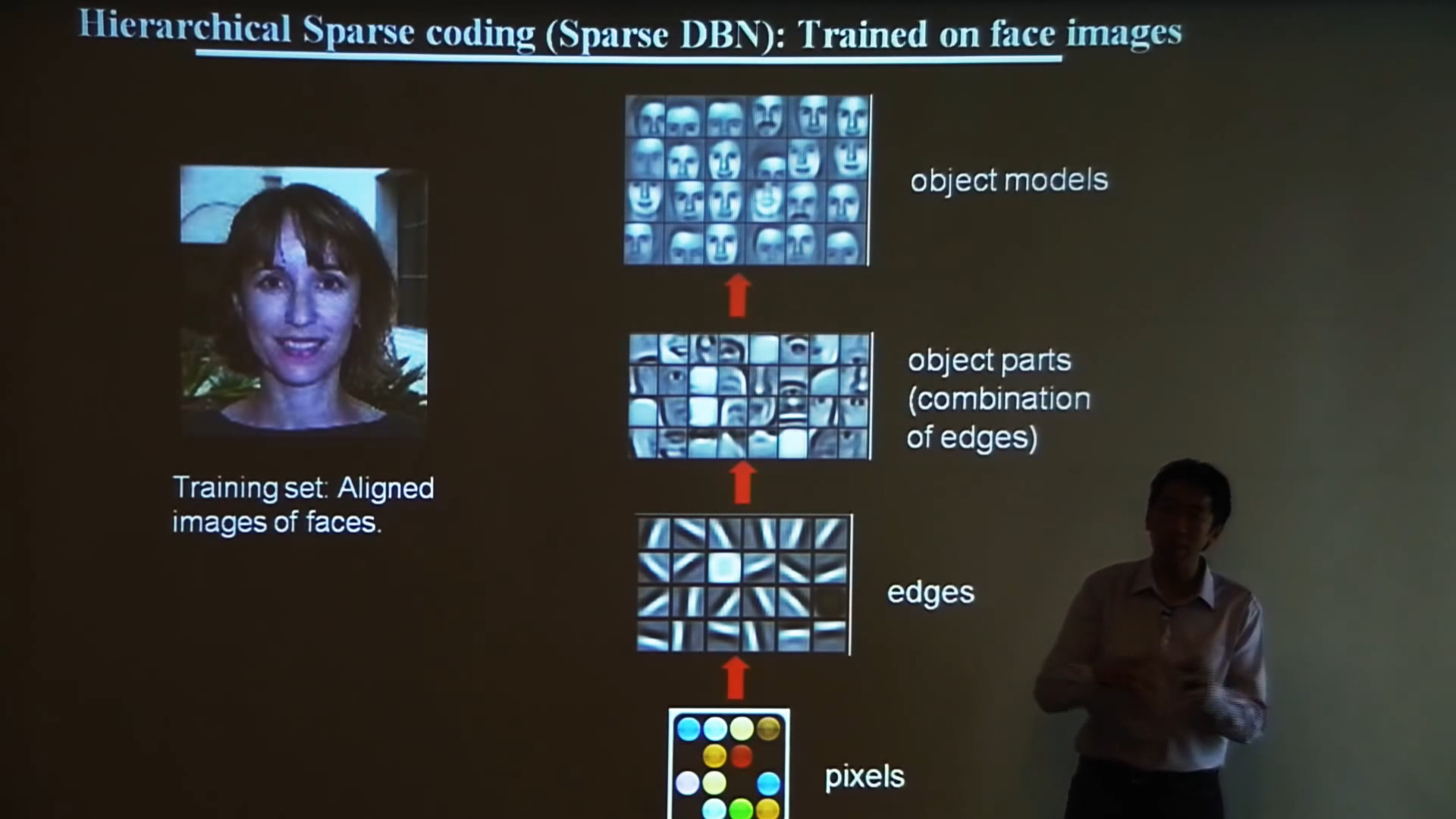
What Andrew Ng is showing in the Deep Learning, Self-Taught Learning and Unsupervised Feature Learning is how the level of abstraction is increasing with each subsequent layer of neurons. For more detailed explanation on this matter I can also recommend Visualizing and Understanding Deep Neural Networks by Matt Zeiler. Anyway, when fine-tuning you will only train the last few layers of the network. The functions below will not only load the model, but will also create a small log file. The log file tf_inception_vars.txt shows all tensorflow variables and indicates which variables would remain unchanged and which would be re-trained through backpropagation in the process of fine-tuning.
def get_init_fn():
    """Returns a function run by the chief worker to warm-start the training."""
    checkpoint_exclude_scopes=["InceptionV3/Logits", "InceptionV3/AuxLogits", "InceptionV3/Mixed_7"]

    exclusions = [scope.strip() for scope in checkpoint_exclude_scopes]

    variables_to_restore = []
    variables_to_retrain = []

    for var in slim.get_model_variables():
        excluded = False
        for exclusion in exclusions:
            if var.op.name.startswith(exclusion):
                excluded = True
                break
        if not excluded:
            variables_to_restore.append(var)
        else:
            variables_to_retrain.append(var)

    with tf.gfile.Open('tf_inception_vars.txt', 'w') as f:
        for var in variables_to_restore:
             f.write('%s ::RESTORED FROM CHECKPOINT\n' % (var))
        for var in variables_to_retrain:
             f.write('%s ::SELECTED FOR RETRAINING\n' % (var))

    return slim.assign_from_checkpoint_fn(
      os.path.join('model','inception_v3.ckpt'), variables_to_restore)
Finally, we select several hyperparameters. A batch size of 128 pictures was a too much for the 12 GB of RAM I dedicated to my Linux VM. 64 was just fine. A single global step needed around 50 seconds. Hence, 1500 steps are around a day of time. If you have a CUDA-capable NVIDIA GPU the training will be much faster. The learning rate is probably the most important hyperparameter. If you choose a learning rate too high, your model will converge very fast without actually learning anything. If you choose a learning rate too low, your model will train just fine, but you may not live long enough to see it finally converged. The Adam Optimizer is the least sensitive Optimizer I have tried out. For this tutorial I started with a learning rate of 0.01 and only after 15 steps (10 min of training) I noticed that the loss does not decrease. A learning rate of 0.001 was just fine. I like the AdamOptimizer as it is very tolerant if you chose a learning rate too high. You can also check this excellent overview on different optimizers.
from inception_v3 import inception_v3
from inception_v3 import inception_v3_arg_scope

TRAIN_SAMPLES = 50000
INCEPTION_IMAGE_SIZE = 299
BATCH_SIZE = 64
NUMBER_OF_STEPS = 1500
LEARNING_RATE = 0.001

slim = tf.contrib.slim

TRAINED_MODEL_DIR = 'inceptionV3_cifar10_finetuned'

with tf.Graph().as_default():
    tf.logging.set_verbosity(tf.logging.INFO)

    train_dataset = get_dataset(
        os.path.join('tfrecord','cifar-10-training-tfrecord'), TRAIN_SAMPLES)

    images, _, labels = load_batch(
       train_dataset, BATCH_SIZE, INCEPTION_IMAGE_SIZE, INCEPTION_IMAGE_SIZE)

    # Create the model, use the default arg scope to configure the batch norm parameters.
    with slim.arg_scope(inception_v3_arg_scope()):
        logits, _ = inception_v3(images, num_classes=train_dataset.num_classes, is_training=True)

    # Specify the loss function:
    one_hot_labels = slim.one_hot_encoding(labels, train_dataset.num_classes)
    slim.losses.softmax_cross_entropy(logits, one_hot_labels)
    total_loss = slim.losses.get_total_loss()

    # Create some summaries to visualize the training process:
    tf.summary.scalar('losses/Total Loss', total_loss)

    # Specify the optimizer and create the train op:
    optimizer = tf.train.AdamOptimizer(learning_rate=LEARNING_RATE)
    train_op = slim.learning.create_train_op(total_loss, optimizer)

    # Run the training:
    final_loss = slim.learning.train(
        train_op,
        logdir=TRAINED_MODEL_DIR,
        init_fn=get_init_fn(),
        number_of_steps=NUMBER_OF_STEPS)

print('Finished training. Last batch loss %f' % final_loss)
INFO:tensorflow:Summary name losses/Total Loss is illegal; using losses/Total_Loss instead.
INFO:tensorflow:Starting Session.
INFO:tensorflow:Starting Queues.
INFO:tensorflow:global_step/sec: 0
INFO:tensorflow:global step 1: loss = 2.9792 (76.37 sec/step)
INFO:tensorflow:global step 2: loss = 2.4563 (52.38 sec/step)
INFO:tensorflow:global step 3: loss = 1.8246 (51.16 sec/step)
INFO:tensorflow:global step 4: loss = 1.9932 (51.35 sec/step)
INFO:tensorflow:global step 5: loss = 1.8377 (49.80 sec/step)
...
INFO:tensorflow:global step 1496: loss = 0.5959 (53.37 sec/step)
INFO:tensorflow:global step 1497: loss = 0.6893 (50.19 sec/step)
INFO:tensorflow:global step 1498: loss = 0.5368 (50.39 sec/step)
INFO:tensorflow:global step 1499: loss = 0.8566 (50.85 sec/step)
INFO:tensorflow:global step 1500: loss = 0.6417 (50.32 sec/step)
INFO:tensorflow:Stopping Training.
INFO:tensorflow:Finished training! Saving model to disk.
Finished training. Last batch loss 0.641681
Evaluation
The neural networks I trained in my last post Convolutional neural network for image classification from scratch was classifying 67% of the images correctly. As there are 10 categories, a random guess would classify 10% of the images correctly. Hence, 67% is quite good. Let’s see…
BATCH_SIZE = 10
TEST_SAMPLE_SIZE = 10000
all_batch_stats = []
def getProbsAsStr(probabilities):
probs_str = 'Probabilities: '
for label, prob in zip(CLASS_NAMES, probabilities):
probs_str += '%s: %.2f%% ' % (label, prob*100)
return probs_str
with tf.Graph().as_default():
tf.logging.set_verbosity(tf.logging.INFO)
test_dataset = get_dataset(
os.path.join('tfrecord','cifar-10-test-tfrecord'), TEST_SAMPLE_SIZE)
images, images_raw, labels = load_batch(
test_dataset, BATCH_SIZE, INCEPTION_IMAGE_SIZE, INCEPTION_IMAGE_SIZE)
# Create the model, use the default arg scope to configure the batch norm parameters.
with slim.arg_scope(inception_v3_arg_scope()):
logits, _ = inception_v3(images, num_classes=test_dataset.num_classes, is_training=True)
probabilities = tf.nn.softmax(logits)
checkpoint_path = tf.train.latest_checkpoint(TRAINED_MODEL_DIR)
init_fn = slim.assign_from_checkpoint_fn(checkpoint_path, slim.get_variables_to_restore())
with tf.Session() as sess:
with slim.queues.QueueRunners(sess):
sess.run(tf.initialize_local_variables())
init_fn(sess)
all_accuracy = []
for i in range(int(TEST_SAMPLE_SIZE/BATCH_SIZE)):
np_probabilities, np_images_raw, np_labels = sess.run([probabilities, images_raw, labels])
all_batch_stats.append((np_labels, np_probabilities))
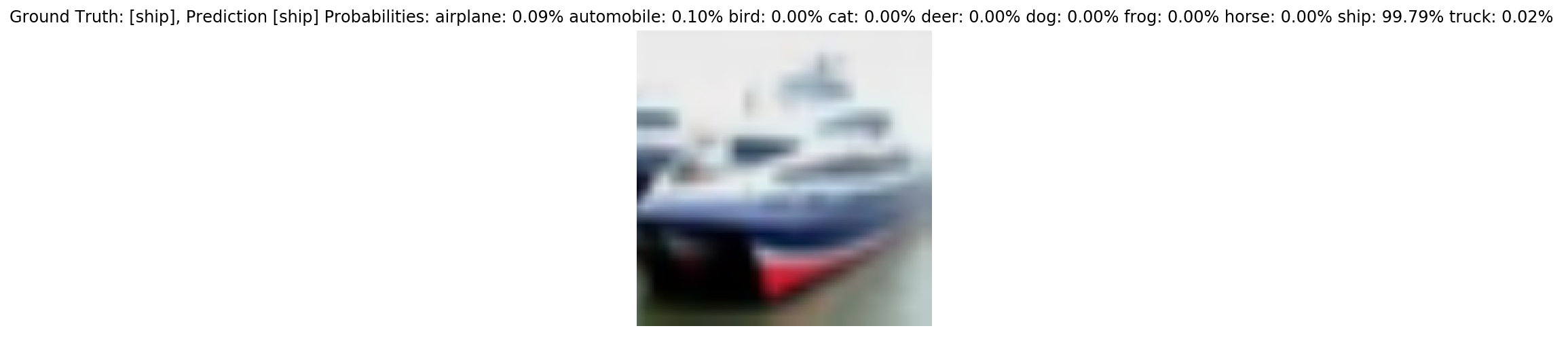
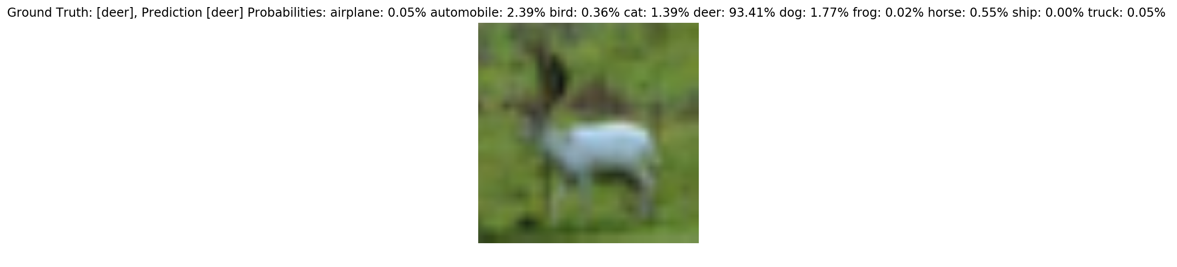
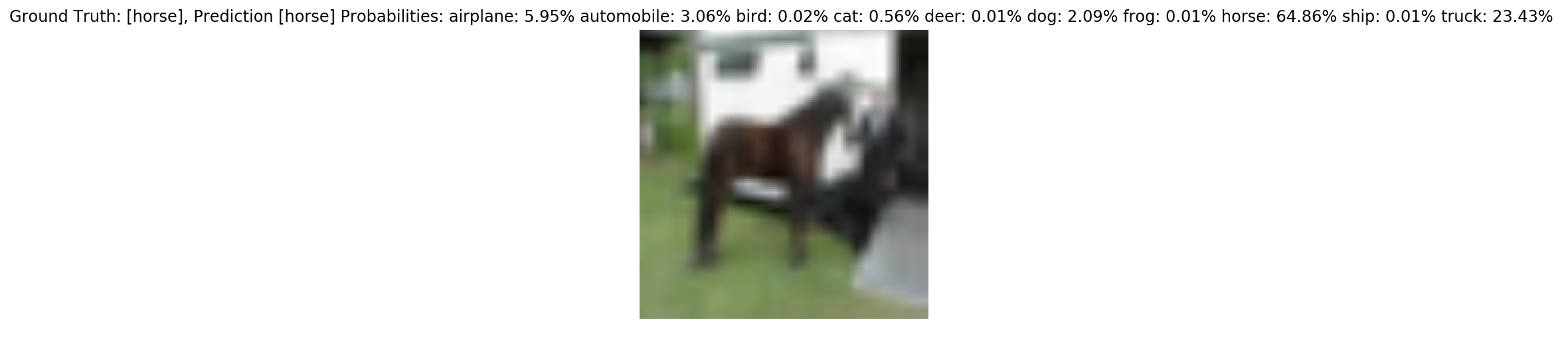
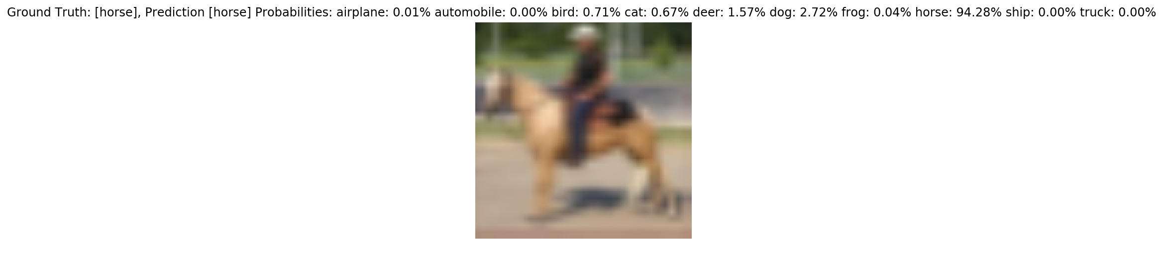
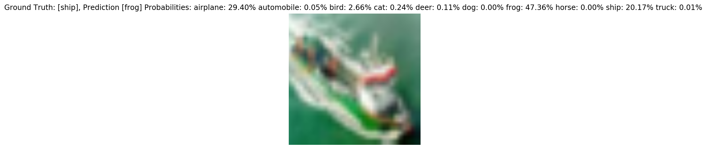
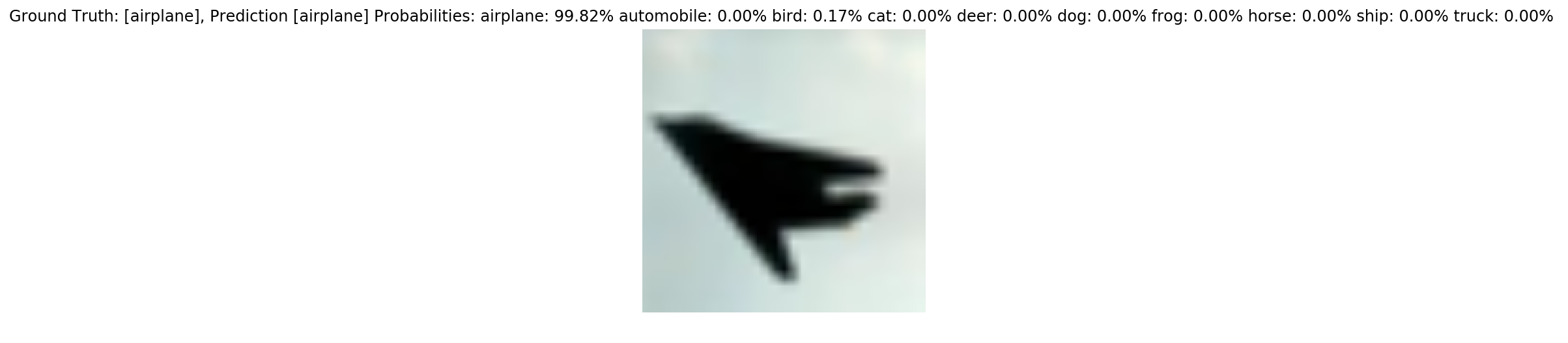
if i == 999: # show images
for j in range(BATCH_SIZE):
image = np_images_raw[j, :, :, :]
true_label = np_labels[j]
predicted_label = np.argmax(np_probabilities[j, :])
predicted_name = test_dataset.labels_to_names[predicted_label]
true_name = test_dataset.labels_to_names[true_label]
plt.figure()
plt.imshow(image.astype(np.uint8))
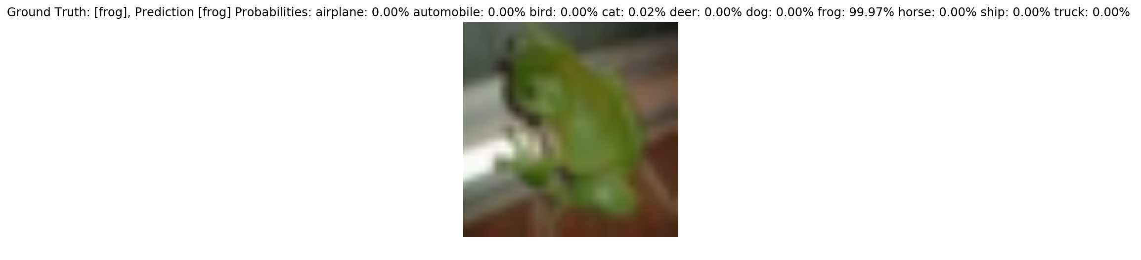
plt.title('Ground Truth: [%s], Prediction [%s] '
% (true_name, predicted_name) + getProbsAsStr(np_probabilities[j, :]))
plt.axis('off')
plt.show()
# Calculate accuracy over the whole test set
all_batch_accuracy = []
for labels, probs in all_batch_stats:
for label, prob in zip(labels, probs):
all_batch_accuracy.append(np.argmax(prob) == label)
print('Overall accuracy', np.mean(all_batch_accuracy))
WARNING:tensorflow:From <ipython-input-36-bcd06166f627>:31: initialize_local_variables (from tensorflow.python.ops.variables) is deprecated and will be removed after 2017-03-02.
Instructions for updating:
Use `tf.local_variables_initializer` instead.
Overall accuracy 0.7985
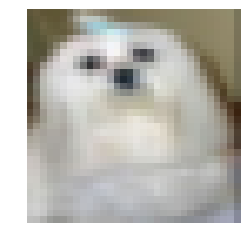
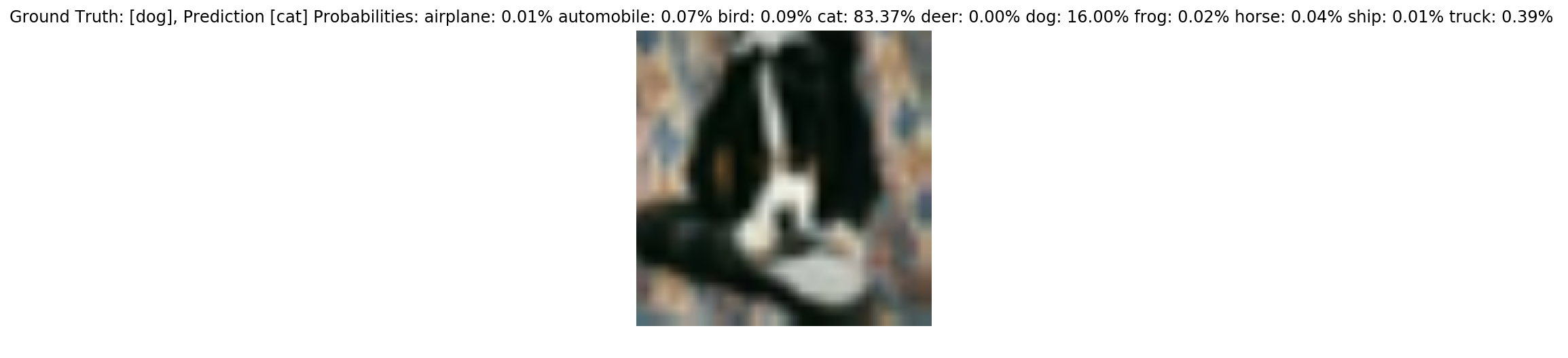
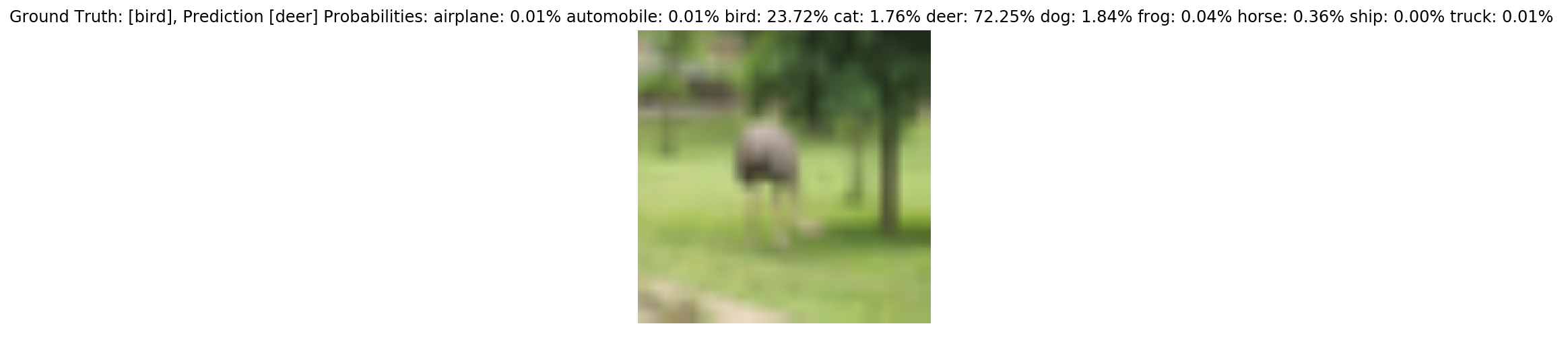
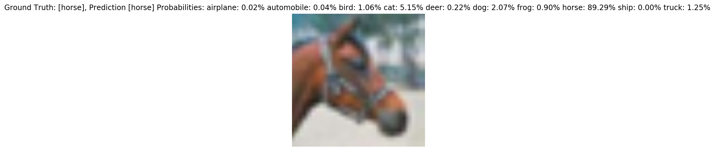
Outlook
Indeed, the accuracy is much better. Evaluated over the whole test set of 10,000 images it is 79,85%. However, there is plenty of room for improvements. While this fine-tuned network will not be at the very bottom of the leaderboard “state of the art in objects classification”, the best model achieves 96.53%. At this point best model is actually better than a human that would achieve an accuracy of only 94%. Look at the fourth image from above that gets incorrectly classified as deer, but is actually a bird. I thought it was a white horse. Here is a link to the whole git repo: cnn-image-classification-cifar-10-inceptionv3.