If you want to truly understand something, you build it from scratch. This post is highly recommended to every software engineer already anticipating Skynet and perceiving AI as some kind of sorcery.
Neural Netowrk from scratch
When designing a neural network machine learning engineers will usually use a high-level library like tensorflow (my personal favorite) or a wrapper on top of tensorflow like keras. And yes, old school ML engineers are still using theano. Having all these tools at your disposal it is rather tempting to view neural networks as a black box and not spend too much time thinking about low-level implementation details like backpropagation, the chain rule, weights initialization, etc. However understanding these concepts might be crucial when fine tuning a neural network. Choosing the optimal count of the hidden layers, the optimal size of each layer, the right activation function, the learning rate, the regularization weights, dropout rate, etc. is not an easy task. Knowing how deep learning works will certainly help you debug and optimize your network. Otherwise, you will be left shooting in the dark, trying to guess the optimal configuration.
In this post I will discuss the my solution to the first assignment in the excellent Udacity program “Deep Learning Nanodegree Foundation”. Before reading any further I strongly recommend watching the video below. It is a very well structured Stanford Lecture on Neural Networks, which is discussing backpropagation and the chain rule:
At 59:07 you can see a very small implementation of a neural network. It is as simple as it gets, it has only an input and an output layer and a single hidden layer between them. Without restricting us to 11 codes of python code, let’s implement a neural network from scratch and run it.
The Data
First, we need some data. Start by downloading the Bike Sharing Dataset. Let’s take a look at the data:
import numpy as np
import pandas as pd
import matplotlib.pyplot as plt

data_path = 'Bike-Sharing-Dataset/hour.csv'
bike_rides = pd.read_csv(data_path)
bike_rides.head()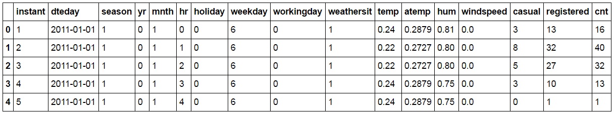
This dataset has the number of riders for each hour of each day from January 1 2011 to December 31 2012. The number of riders is split between casual and registered, summed up in the cnt column. You can see the first few rows of the data on the image above.
Let’s plot the number of bike riders over the first 20 days in the data set.
rides[:24*20].plot(x='dteday', y='cnt')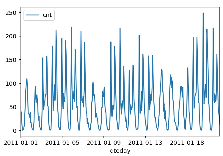
You can see the hourly rentals here. This data is pretty complicated! The weekends have lower overall ridership and there are spikes when people are biking to and from work during the week. Looking at the data above, we also have information about temperature, humidity, and windspeed, all of this likely affecting the number of riders. The neural network will by trying to capture all these.
Let’s convert categorical data into binary, so that it can be used as input in the neural network:
dummy_fields = ['season', 'weathersit', 'mnth', 'hr', 'weekday']
for each in dummy_fields:
    dummies = pd.get_dummies(bike_rides[each], prefix=each, drop_first=False)
    bike_rides = pd.concat([bike_rides, dummies], axis=1)

fields_to_drop = ['instant', 'dteday', 'season', 'weathersit',
                  'weekday', 'atemp', 'mnth', 'workingday', 'hr']
data = bike_rides.drop(fields_to_drop, axis=1)
data.head()
To make the neural network converge faster, let’s standardize each of the continuous variables. That is, we’ll shift and scale the variables such that they have zero mean and a standard deviation of 1. Also known as standard scaling.
from sklearn.preprocessing import StandardScaler
quant_features = ['casual', 'registered', 'cnt', 'temp', 'hum', 'windspeed']
data.loc[:, quant_features] = StandardScaler().fit_transform(data[quant_features])
Let’s save the last 21 days of the data to use as a test set after the network is trained. The test set is going to be used to make predictions and compare them with the actual number of riders.
# Save the last 21 days
test_data = data[-21*24:]
data = data[:-21*24]

# Separate the data into features and targets
target_fields = ['cnt', 'casual', 'registered']
features, targets = data.drop(target_fields, axis=1), data[target_fields]
test_features, test_targets = test_data.drop(target_fields, axis=1), test_data[target_fields]
The Neural Network (pure magic)
Usually, you would like to make one more split and create a validation set in order to observe and control the bias and variance of the neural network. Although this is EXTREMELY important, I will skip this step here, as I want to focus on the network implementation. If you want to learn more about identifying and controlling bias and variance you can take a look at Andrew NG’s lecture Machine learning W6 4 Diagnosing Bias vs Variance.
So let’s implement the neural network:
class NeuralNetwork:
    def __init__(self, input_nodes, hidden_nodes, output_nodes, learning_rate):
        # Set number of nodes in input, hidden and output layers.
        self.input_nodes = input_nodes
        self.hidden_nodes = hidden_nodes
        self.output_nodes = output_nodes

        # Initialize weights
        self.weights_input_to_hidden = np.random.normal(0.0, self.hidden_nodes**-0.5,
                                                (self.hidden_nodes, self.input_nodes))

        self.weights_hidden_to_output = np.random.normal(0.0, self.output_nodes**-0.5,
                                                (self.output_nodes, self.hidden_nodes))

        self.learning_rate = learning_rate

        #### Set this to your implemented sigmoid function ####
        # Activation function is the sigmoid function
        self.activation_function = lambda x: 1 / (1 + np.exp(-x))

    def train(self, inputs_list, targets_list):
        # Convert inputs list to 2d array
        inputs = np.array(inputs_list, ndmin=2).T
        targets = np.array(targets_list, ndmin = 2).T

        #### Implement the forward pass here ####
        ### Forward pass ###
        # Hidden layer
        # signals into hidden layer
        hidden_inputs =  self.weights_input_to_hidden.dot(inputs)
        # signals from hidden layer
        hidden_outputs = self.activation_function(hidden_inputs)

        # Output layer
        # signals into final output layer
        final_inputs = self.weights_hidden_to_output.dot(hidden_outputs)
        # signals from final output layer
        final_outputs = final_inputs

        #### Implement the backward pass here ####
        ### Backward pass ###

        # Output error
        # Output layer error is the difference between desired target and actual output.
        output_errors = targets - final_outputs

        # This is the most IMPORTANT part!
        # The error is been backpropagated to the hidden layer
        # By using the chain rule one can calculate the
        # errors propagated to the hidden layer and then the
        # hidden layer gradients
        hidden_errors = output_errors.dot(self.weights_hidden_to_output)
        hidden_grad = hidden_errors.T * hidden_outputs * (1-hidden_outputs)

        # :Update the weights
        # update hidden-to-output weights with gradient descent step
        self.weights_hidden_to_output += self.learning_rate * output_errors.dot(hidden_outputs.T)
        # update input-to-hidden weights with gradient descent step
        self.weights_input_to_hidden += self.learning_rate * hidden_grad.dot(inputs.T)

    def run(self, inputs_list):
        # Run a forward pass through the network
        inputs = np.array(inputs_list, ndmin=2).T

        #### Implement the forward pass here ####
        # Hidden layer
        # signals into hidden layer
        hidden_inputs =  self.weights_input_to_hidden.dot(inputs)
        # signals from hidden layer)
        hidden_outputs = self.activation_function(hidden_inputs)

        # Output layer
        # signals into final output layer
        final_inputs = self.weights_hidden_to_output.dot(hidden_outputs)
        # signals from final output layer
        final_outputs = final_inputs

        return final_outputs
Let’s train the network. It takes a couple of minutes…
### You can change the hyperparameters here ###
epochs = 5000
learning_rate = 0.01
hidden_nodes = 10
output_nodes = 1

N_i = features.shape[1]
network = NeuralNetwork(N_i, hidden_nodes, output_nodes, learning_rate)

train_loss_progress = []
for e in range(epochs):
    # Go through a random batch of 128 records from the training data set
    batch = np.random.choice(features.index, size=128)
    for record, target in zip(features.ix[batch].values,
                              targets.ix[batch]['cnt']):
        network.train(record, target)

    if e%(epochs/10) == 0:
        # Calculate losses for the training and test sets
        loss = MSE(network.run(features), targets['cnt'].values)
        train_loss_progress.append(loss)
        print('Training loss: {:.4f}'.format(loss))

plt.plot(losses['train'], label='Training loss')
plt.legend()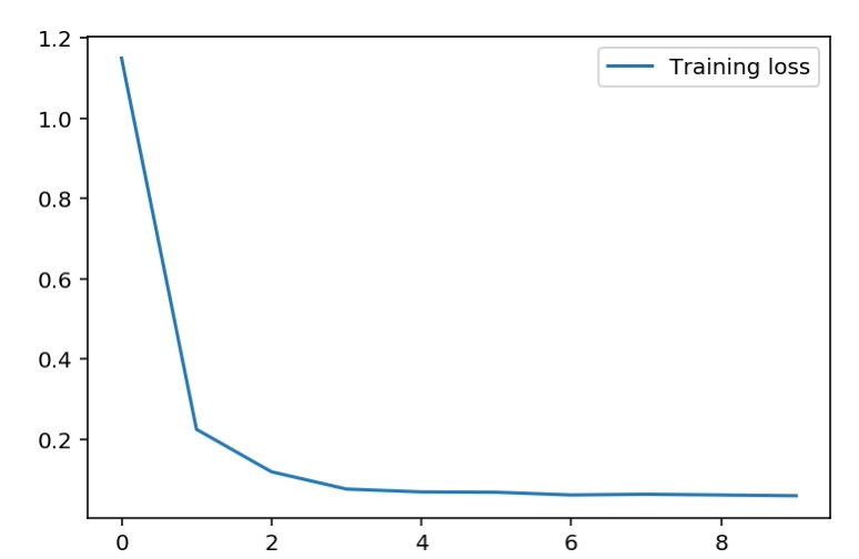
Let’s check how well the data is being predicted:
fig, ax = plt.subplots(figsize=(8,4))

mean, std = scaled_features['cnt']
predictions = network.run(test_features)*std + mean
ax.plot(predictions[0], label='Prediction')
ax.plot((test_targets['cnt']*std + mean).values, label='Data')
ax.set_xlim(right=len(predictions))
ax.legend()

dates = pd.to_datetime(bike_rides.ix[test_data.index]['dteday'])
dates = dates.apply(lambda d: d.strftime('%b %d'))
ax.set_xticks(np.arange(len(dates))[12::24])
_ = ax.set_xticklabels(dates[12::24], rotation=45)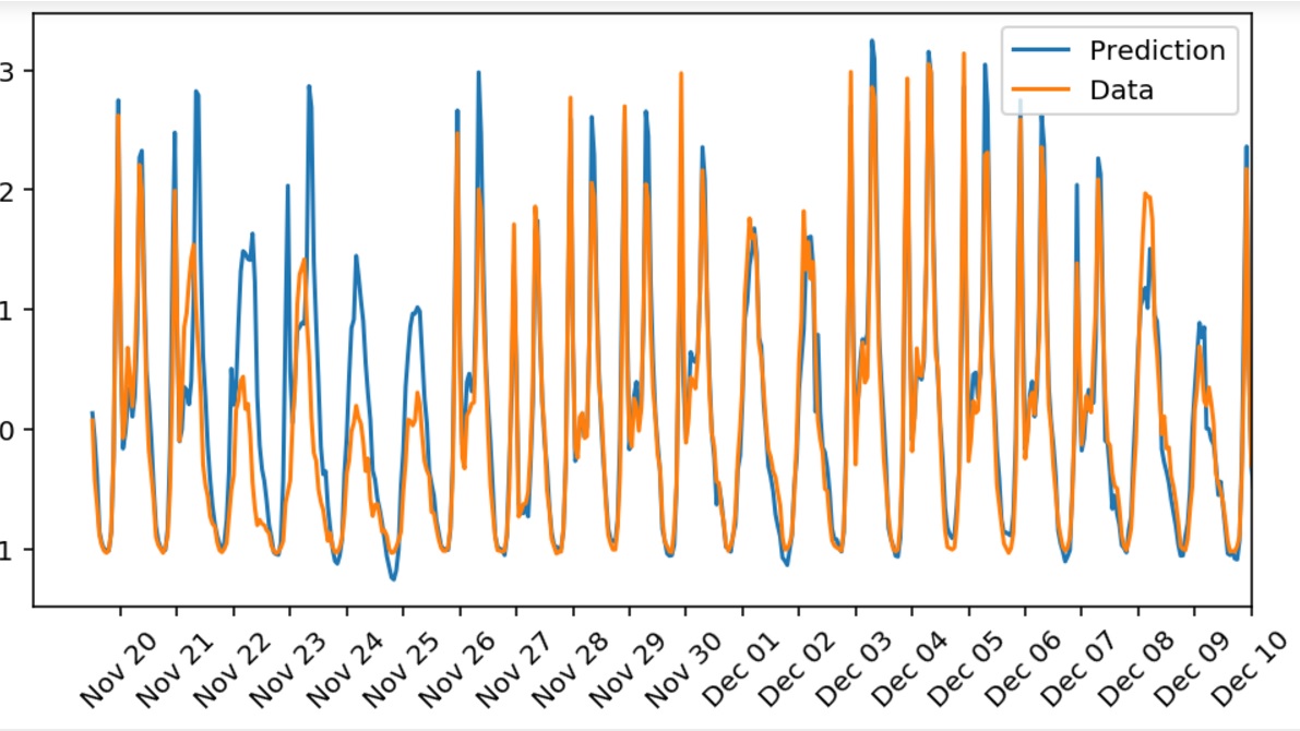
As you can see, you can easily implement a neural network from scratch that could get you pretty decent predictions for some real world problems. Nevertheless, there is a long way to go since Skynet is operational.